Predicting Seismic Activity Using Dense Acceleration Data

• 

  Log-likelihood

Title: Predicting Seismic Activity Using Dense Acceleration Data and RNNs

Benjamin Pomeranz (bjpomera), Bentzion Gitig(bgitig), Armaan Patankar(ampatank), Skylar Walters (swalter4)

Introduction

The primary challenge we are approaching here is forecasting earthquakes, or more generally predicting ground acceleration. At present, earthquakes are often hard to predict on a short-term or long-term basis; the technique we will be employing revolves around examining historical data and making probabilistic predictions for the next earthquake event given some window of prior events.

We are basing our paper on Using Deep Learning for Flexible and Scalable Earthquake Forecasting, by Dascher-Cousineau et al. 2023. In this paper, the group introduced the Recurrent Earthquake foreCAST (RECAST) model to predict the probability of an earthquake in a given time interval using larger datasets than have been leveraged in the past. This model will therefore output a probability distribution describing the probability of a tremor event over a given timeframe, given a history of past earthquake events. Critically, we will be implementing our version of the RECAST model with slightly differing goals. We will not be using a simulated dataset as the research team did, but rather use a new dataset, which has yet to be examined using machine learning techniques. This dataset contains ground micro-electro-mechanical accelerometer data recorded continuously between 2017 and 2020, which we will refer to as the Grillo dataset. As it is a dataset containing near continuous acceleration data over a much more precise timescale, as opposed to sparser data with only time labels and richter magnitudes, we will emphasize a) predicting smaller, more sensitive tremors and b) having shorter-scale forecasting times (eg. predicting an earthquake minutes to hours in advance).

We selected this paper after discovering the Grillo dataset. We saw that it has yet to have been explored in-depth using machine learning or deep learning techniques. As such, we hoped to be the first to fully take advantage of its ample data (each second has 30-100 data points, taken over 3 years). The team found this paper to be particularly interesting as a means of using the data, as our dataset structures are somewhat similar, but very different in their timeframes, data precision, and robustness.

This project will be a regression task. The mode will take in time, magnitude, and acceleration data for a given timeframe, then output a probability density function and survival function describing the likelihood of a tremor event over a given time interval (i.e. next one minute, next one day, next 5 days, next 15 days, etc.).

Related Work A piece of related work to our project is Structural Damage Prediction from Earthquakes Using Deep Learning, Sharma et al. 2024. This paper implements a structural health monitoring system (SHM), which assesses the damage to structures over their life cycles, based on accelerometer data to detect damage from earthquakes. It includes a number of approaches, including with 1D and 2D CNNs as well as one with an LSTM. In the 1D CNN and LSTM approaches, the model was trained on the accelerometer data. The heat maps of each of the previous approaches’ training data was used as the training input for the 2D CNN-based approach. This paper found that the 1D CNN was the most effective model for SHM prediction when working with accelerometer data. Additional prior work: https://ieeexplore.ieee.org/document/9509429 Similar to our paper, however it works on earthquake detection instead of forecasting. Data difference: uses “earthquake notifications” instead of acceleration at timesteps Public implementations: https://zenodo.org/records/8161777 - from original paper

Data https://github.com/openeew/openeew/tree/master/data Our dataset diverges notably from the data in the paper. That study used simulated datasets as well as real-world data, with each data point consisting only of a time and magnitude. Moreover, it covers a 40 year timespan even in the real world data. However, we are using a dataset over a 6-year timespan. As a result, we are anticipating predicting a) less large earthquakes (eg. focusing on the prediction of smaller tremors) and thus b) potentially shorter prediction times (eg. less “advanced” notice for the tremor). Our data comes from the Grillo/IBM/Linux OpenEEW dataset, which is available on AWS. Each sensor in the dataset measures three axes of acceleration, in Gs, updated 30-100 times per second, from 2017 until today. This data comes in 5 minute blocks, each located in a JSON file, but can be processed en masse with AWS tools. There are 27 of these sensors located across the Southwest coast of Mexico. From 2017 to 2021, there were about 750 earthquakes of Richter magnitude >3.5 in this area. Thus, if we only include those earthquakes as our events, we can preprocess this data into 1200-1500 events of magnitude 3.5, (and even more than that if we lower the required magnitude), and with each of these data points we can include the time of the event, the magnitude of the event as derived from the acceleration, and the acceleration in the vertical direction within a time period of length X starting from the beginning of the earthquake. Approximate conversion of acceleration into Mercalli scale and then Richter scale is not uncommon. We are still deciding how long X should be. Additionally, we can parallelize this training across the 27 locations to have up to 35,000 data points. We also have to process the data to get our labels, which for each event would be the time interval between the event E(i) and the following event E(i+1), but once we have processed our data into the form (time of event, magnitude of event, acceleration matrix for event), this should be fairly easy. See here for Python EEW interface to download data for a given time period, from a given set of devices: https://github.com/openeew/openeew-python.

Methodology

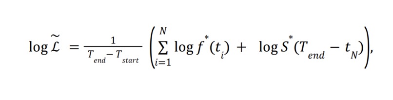
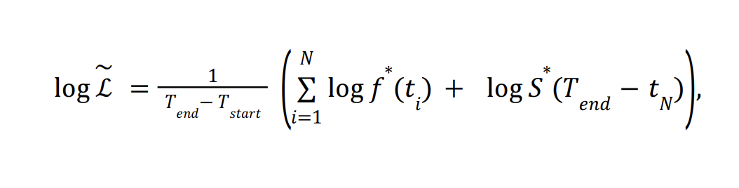
Our model will be very similar to the original RECAST model, although we plan to reimplement all elements of the model in TensorFlow, as opposed to the original Pytorch, when creating our own model. In the original paper, the model is primarily a GRU RNN where the input at each time step t is: (log(Ti-T(i-1)-average time interval, Mi - average Magnitude) where Ti is the time of an event and Mi is the magnitude of an event. They write in the original paper, “If other features (e.g., locations) are available, they can be ‾ concatenated with 𝑦 .” At the most basic level, that is what we plan to do. However, because there is such a wealth of acceleration data, we will play with several methods of implementing it in the model. We plan to include wholesale vectors of acceleration over a given time period around the seismic event in one implementation, but also to include a CNN in another which could ideally extract features from the acceleration data which would better allow the RNN to predict a distribution of future events. We believe that this added information, of not only magnitude of a given event but also of near continuous acceleration data for some amount of time surrounding the event, could potentially greatly increase the efficacy of the model in predicting future seismic activity.At each time step, the hidden state outputted by the RNN is used to compute a PDF of the time of the next event in the original paper, by outputting parameters P1,...,Pn which are used to generate a mixed Weibull Distribution, f*(t), which gives the probability density of the amount of time to the next event, or in other words the inter event time interval. Then, the log likelihood function is computed as follows against the PDF in attached image screenshot.

An alternate option: Analyze the distribution of inter event times, and make it into a categorization problem - have the model assign a probability to each range of inter event times at each step. We, like the original paper, plan to maximize the log-likelihood of Recast on the training set by performing gradient ascent with Adam on the model parameters with a learning rate of 0.01. To avoid overfitting, after each epoch, we evaluate the log-likelihood of the model on a validation set and stop training once the validation objective stops improving. We allow for a maximum of [500?] training epochs and perform early stopping if the validation loss does not improve in the last 200 epochs. After training, we recover the parameters of the model with the best performance on the validation set. It seems likely that the hardest part of working with this implementation will be learning how to work with the Weibull Distributions and training the model based off of the distributions they parameterize. We plan to rely heavily on the source code of the original paper to gain better understanding of how this can be implemented, and to do so in Tensor Flow.

Metrics

The RECAST paper hoped to illustrate that patterns in seismic data could be recognized by a temporal point process model, and they wanted to prove this by comparing it to a previous seismic prediction model, ETAS. Similarly, we hope to show that by incorporating underutilized accelerometer data, we can improve on the usage of RNNs to understand patterns in seismic data. We can very easily compare our model’s output with the original RECAST Model using Log Likelihood Ratio: Log-Likelihood(our model) - Log-Likelihood(RECAST). This will all be evaluated on testing data that neither model will be trained on. Log likelihood is defined in the original paper as follows, where S* is the probability the model gives that there will be no events between T(end) and t(N). This is similar to a continuous categorical cross entropy. Again, see attached image. Both models will be trained on the OpenEEW data of smaller earthquakes, so we can see how the modified RECAST model compares to the original in an even playing field. There aren’t many very intuitive accuracy metrics for this task, since it is outputting a distribution, so comparing it to the effectiveness of other models will still be a primary accuracy metric. Of course, we also want to see how our model can actually transfer to the real world. Another accuracy metric we will compute is, on average, how likely did our prediction pdf say (within the range of a given confidence interval), that the next event would occur when it did. Because the Mixed Weibull Distributions have a closed form for CDF, confidence intervals can be easily computed. We can test this across different confidences.We can easily compute the odds that there is an event before or after a given time, and so perhaps a metric we could use is predicting whether there will be an event in the next day/2 days/5 days/etc., and use a more classic accuracy metric such as categorical accuracy for these predictions across different levels of confidence. Base goal: almost as good as RECAST in terms of log-likelihood (so a ratio slightly less than 1 - say .9) when trained on this data. Target goal: Given its additional information intake (acceleration vector), a target goal would be for our model to outperform RECAST on the task of modeling seismic activity, as measured by log-likelihood. Stretch goal: If we have time and ability to also implement forecasting with this model, such that the RNN can predict and thus generate its own synthetic acceleration/time data, which RECAST does do, that would be excellent.

Ethics

The primary ethical concerns regarding our model revolve around the implications of false positives and false negatives.

Key stakeholders in this problem are the individuals living in the areas where an earthquake is predicted to occur. Having advanced warning systems for earthquakes can ensure residents evacuate in a timely manner, saving lives in the process. Additional stakeholders could be construction and insurance companies. Having more robust information on when major earthquakes may occur will likely lead to changes in pricing for home insurance, while construction companies may begin to build with more earthquake consideration in mind. These impacts, in turn, will once again affect the resident stakeholders: rising cost of insurance and costs for repairs could push out some residents. The issue of inaccurate predictions would be particularly harmful to the resident stakeholders. If we predict earthquakes with too high of a frequency (eg. have false positives), then residents would be less likely to trust a true earthquake “alarm.” In turn, they would be less likely to evacuate an area, resulting in potential loss of life. If we were to predict earthquakes with too low of a frequency, then we risk missing potentially-dangerous earthquakes that would likewise result in harm.

This nuance in the dangers of false predictions for stakeholders plays into the importance of quantifying error and success. We plan on quantifying success largely through comparisons with another model, as well as evaluating how accurate our PDF outputs are at different confidence intervals. Confidence intervals specifically have a big trade off - the more accurate the information we provide to people, the less precise it is. This slope becomes slippery very fast - if people are able to learn with confidence that they may experience a tremor in a range between 1 and 18 days, that is not particularly actionable. Conversely, having a ⅓ shot of an earthquake during a one hour interval is not very motivating to most people.

Division of Labor

• This section is largely still being discussed, and very open to change as we continue working on the project more * Data Analysis and imaging: Armaan/Bentzi Data preprocessing: Ben/Skylar Model construction: Everyone Adding accuracy metrics: Ben Ablation and tweaking: Bentzi/Skylar/Armaan

Built With

• python
• tensorflow